import io, os, sys, types, time, datetime, math, random, requests, subprocess, tempfile from io import StringIO, BytesIO
Packages Install
We’ll now install a few more libraries. This is an easy way to install libraries in a way that are recognised and managed by conda. Do this once and then comment it out for subsequent runs.
There’s a lot of packages available to us, and most of them were installed when running the dockerfile that created the docker instance. Let’s make sure they are all up to date. Do this once and then comment it out for subsequent runs.
1
#!conda update --yes --all
Packages Import
These are all the packages we’ll be using. Importing individual libraries make it easy for us to use them without having to call the parent libraries.
# Data Manipulation import numpy as np import pandas as pd
# Visualization import matplotlib.pyplot as plt import missingno import seaborn as sns from pandas.plotting import scatter_matrix from mpl_toolkits.mplot3d import Axes3D
# Feature Selection and Encoding from sklearn.feature_selection import RFE, RFECV from sklearn.svm import SVR from sklearn.decomposition import PCA from sklearn.preprocessing import OneHotEncoder, LabelEncoder, label_binarize
# Machine learning import sklearn.ensemble as ske from sklearn import datasets, model_selection, tree, preprocessing, metrics, linear_model from sklearn.svm import LinearSVC from sklearn.ensemble import RandomForestClassifier, GradientBoostingClassifier from sklearn.neighbors import KNeighborsClassifier from sklearn.naive_bayes import GaussianNB from sklearn.linear_model import LinearRegression, LogisticRegression, Ridge, Lasso, SGDClassifier from sklearn.tree import DecisionTreeClassifier import tensorflow as tf
# Grid and Random Search import scipy.stats as st from scipy.stats import randint as sp_randint from sklearn.model_selection import GridSearchCV from sklearn.model_selection import RandomizedSearchCV
# Metrics from sklearn.metrics import precision_recall_fscore_support, roc_curve, auc
Let’s download the data and save it to a folder in our local directory called ‘dataset’. Download it once, and then comment the code out for subsequent runs.
After downloading the data, we load it directly from Disk into a Pandas Dataframe in Memory. Depending on the memory available to the Docker instance, this may be a problem.
The data comes separated into the Training and Test datasets. We will join the two for data exploration, and then separate them again before running our algorithms.
# Displaying the size of the Dataframe in Memory defconvert_size(size_bytes): if size_bytes == 0: return"0B" size_name = ("Bytes", "KB", "MB", "GB", "TB", "PB", "EB", "ZB", "YB") i = int(math.floor(math.log(size_bytes, 1024))) p = math.pow(1024, i) s = round(size_bytes / p, 2) return"%s %s" % (s, size_name[i]) convert_size(dataset_raw.memory_usage().sum())
'5.59 MB'
Data Exploration - Univariate
When exploring our dataset and its features, we have many options available to us. We can explore each feature individually, or compare pairs of features, finding the correlation between. Let’s start with some simple Univariate (one feature) analysis.
Features can be of multiple types:
Nominal: is for mutual exclusive, but not ordered, categories.
Ordinal: is one where the order matters but not the difference between values.
Interval: is a measurement where the difference between two values is meaningful.
Ratio: has all the properties of an interval variable, and also has a clear definition of 0.0.
There are multiple ways of manipulating each feature type, but for simplicity, we’ll define only two feature types:
Numerical: any feature that contains numeric values.
Categorical: any feature that contains categories, or text.
1
2
# Describing all the Numerical Features dataset_raw.describe()
age
fnlwgt
education-num
capital-gain
capital-loss
hours-per-week
count
48842.000000
4.884200e+04
48842.000000
48842.000000
48842.000000
48842.000000
mean
38.643585
1.896641e+05
10.078089
1079.067626
87.502314
40.422382
std
13.710510
1.056040e+05
2.570973
7452.019058
403.004552
12.391444
min
17.000000
1.228500e+04
1.000000
0.000000
0.000000
1.000000
25%
28.000000
1.175505e+05
9.000000
0.000000
0.000000
40.000000
50%
37.000000
1.781445e+05
10.000000
0.000000
0.000000
40.000000
75%
48.000000
2.376420e+05
12.000000
0.000000
0.000000
45.000000
max
90.000000
1.490400e+06
16.000000
99999.000000
4356.000000
99.000000
1
2
# Describing all the Categorical Features dataset_raw.describe(include=['O'])
workclass
education
marital-status
occupation
relationship
race
sex
native-country
predclass
count
46043
48842
48842
46033
48842
48842
48842
47985
48842
unique
8
16
7
14
6
5
2
41
4
top
Private
HS-grad
Married-civ-spouse
Prof-specialty
Husband
White
Male
United-States
<=50K
freq
33906
15784
22379
6172
19716
41762
32650
43832
24720
1 2
# Let's have a quick look at our data dataset_raw.head()
age
workclass
fnlwgt
education
education-num
marital-status
occupation
relationship
race
sex
capital-gain
capital-loss
hours-per-week
native-country
predclass
0
39
State-gov
77516
Bachelors
13
Never-married
Adm-clerical
Not-in-family
White
Male
2174
0
40
United-States
<=50K
1
50
Self-emp-not-inc
83311
Bachelors
13
Married-civ-spouse
Exec-managerial
Husband
White
Male
0
0
13
United-States
<=50K
2
38
Private
215646
HS-grad
9
Divorced
Handlers-cleaners
Not-in-family
White
Male
0
0
40
United-States
<=50K
3
53
Private
234721
11th
7
Married-civ-spouse
Handlers-cleaners
Husband
Black
Male
0
0
40
United-States
<=50K
4
28
Private
338409
Bachelors
13
Married-civ-spouse
Prof-specialty
Wife
Black
Female
0
0
40
Cuba
<=50K
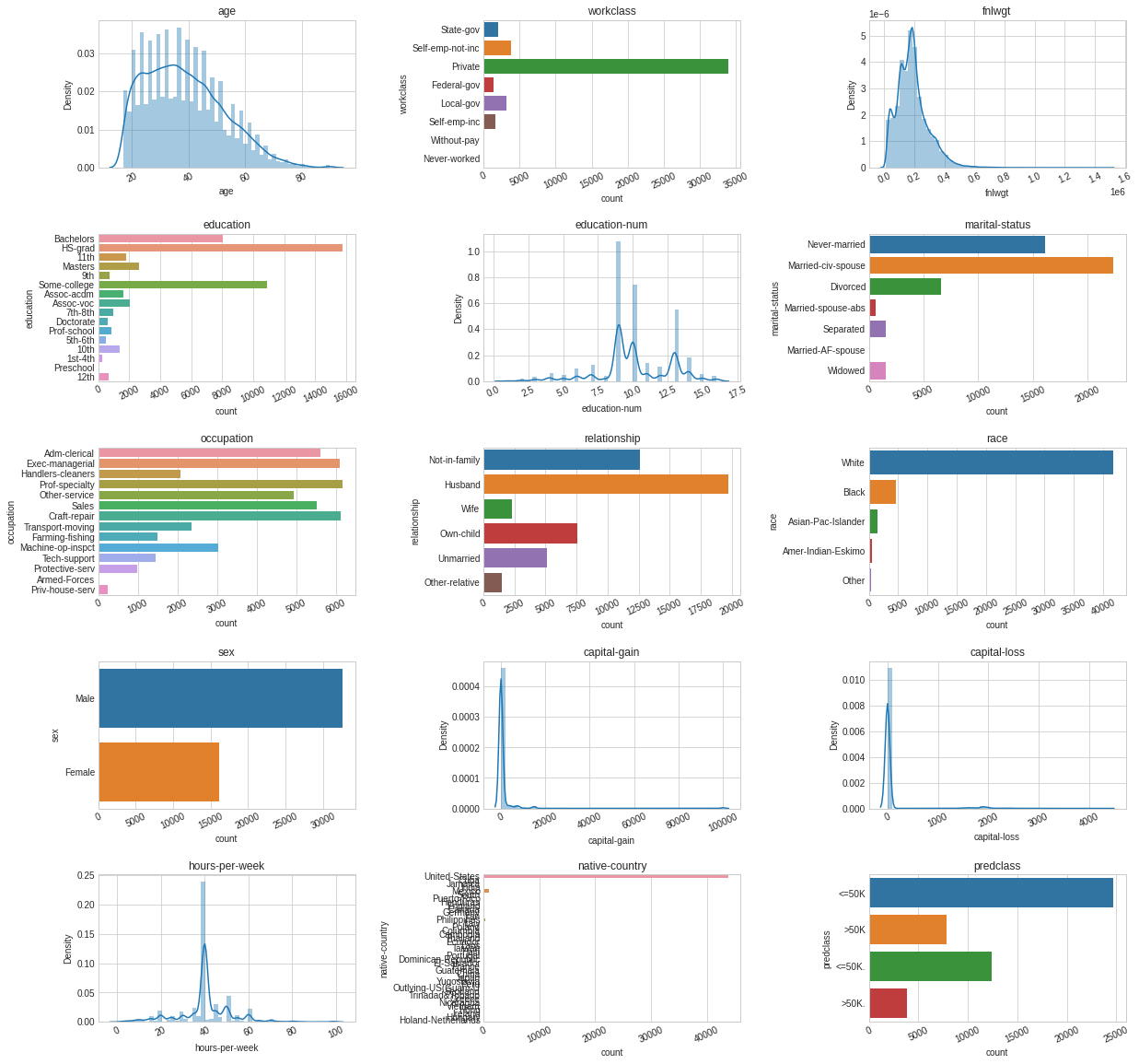
1 2 3 4 5 6 7 8 9 10 11 12 13 14 15 16 17 18 19
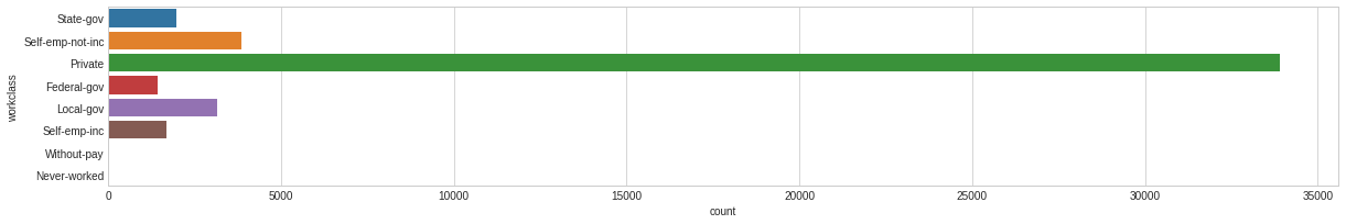
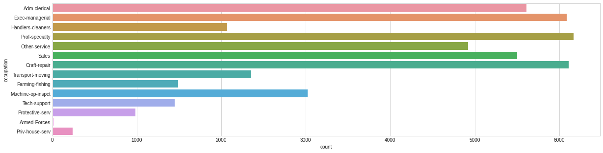
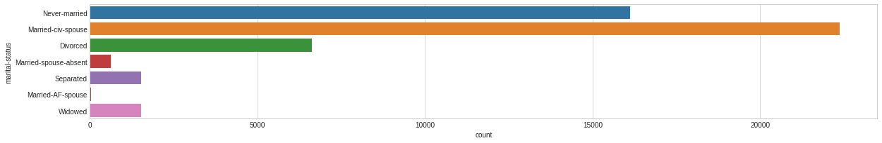
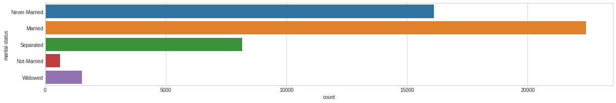
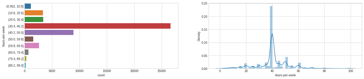
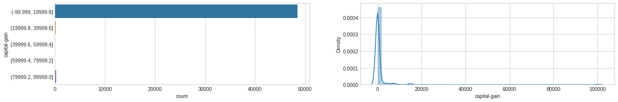
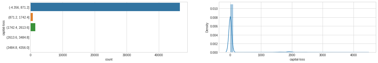
# Let’s plot the distribution of each feature defplot_distribution(dataset, cols=5, width=20, height=15, hspace=0.2, wspace=0.5): plt.style.use('seaborn-whitegrid') fig = plt.figure(figsize=(width,height)) fig.subplots_adjust(left=None, bottom=None, right=None, top=None, wspace=wspace, hspace=hspace) rows = math.ceil(float(dataset.shape[1]) / cols) for i, column in enumerate(dataset.columns): ax = fig.add_subplot(rows, cols, i + 1) ax.set_title(column) if dataset.dtypes[column] == np.object: g = sns.countplot(y=column, data=dataset) substrings = [s.get_text()[:18] for s in g.get_yticklabels()] g.set(yticklabels=substrings) plt.xticks(rotation=25) else: g = sns.distplot(dataset[column]) plt.xticks(rotation=25) plot_distribution(dataset_raw, cols=3, width=20, height=20, hspace=0.45, wspace=0.5)
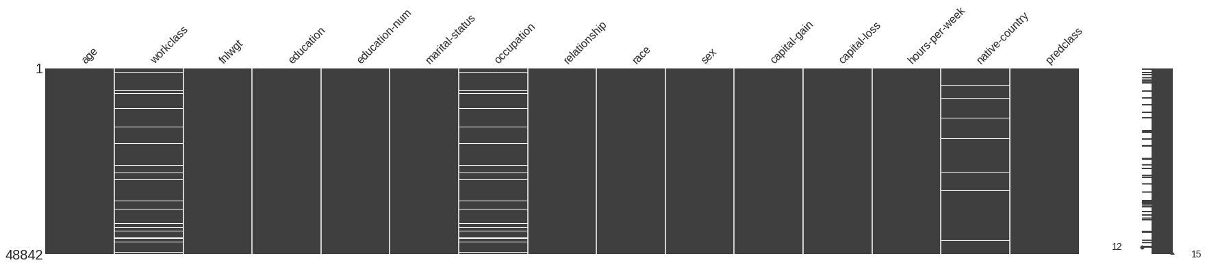
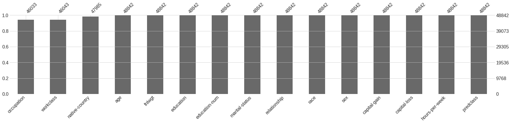
1 2
# How many missing values are there in our dataset? missingno.matrix(dataset_raw, figsize = (30,5))
Cleaning: To clean our data, we’ll need to work with:
Missing values: Either omit elements from a dataset that contain missing values or impute them (fill them in).
Special values: Numeric variables are endowed with several formalized special values including ±Inf, NA and NaN. Calculations involving special values often result in special values, and need to be handled/cleaned.
Outliers: They should be detected, but not necessarily removed. Their inclusion in the analysis is a statistical decision.
Obvious inconsistencies: A person’s age cannot be negative, a man cannot be pregnant and an under-aged person cannot possess a drivers license. Find the inconsistencies and plan for them.
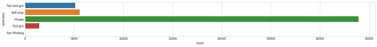
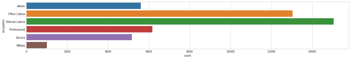
Engineering: There are multiple techniques for feature engineering:
Decompose: Converting 2014-09-20T20:45:40Z into categorical attributes like hour_of_the_day, part_of_day, etc.
Discretization: We can choose to either discretize some of the continuous variables we have, as some algorithms will perform faster. We are going to do both, and compare the results of the ML algorithms on both discretized and non discretised datasets. We’ll call these datasets:
dataset_bin => where Continuous variables are Discretised
dataset_con => where Continuous variables are Continuous
Reframe Numerical Quantities: Changing from grams to kg, and losing detail might be both wanted and efficient for calculation
Feature Crossing: Creating new features as a combination of existing features. Could be multiplying numerical features, or combining categorical variables. This is a great way to add domain expertise knowledge to the dataset.
Imputation: We can impute missing values in a number of different ways:
Hot-Deck: The technique then finds the first missing value and uses the cell value immediately prior to the data that are missing to impute the missing value.
Cold-Deck: Selects donors from another dataset to complete missing data.
Mean-substitution: Another imputation technique involves replacing any missing value with the mean of that variable for all other cases, which has the benefit of not changing the sample mean for that variable.
Regression: A regression model is estimated to predict observed values of a variable based on other variables, and that model is then used to impute values in cases where that variable is missing.
1 2 3
# To perform our data analysis, let's create new dataframes. dataset_bin = pd.DataFrame() # To contain our dataframe with our discretised continuous variables dataset_con = pd.DataFrame() # To contain our dataframe with our continuous variables
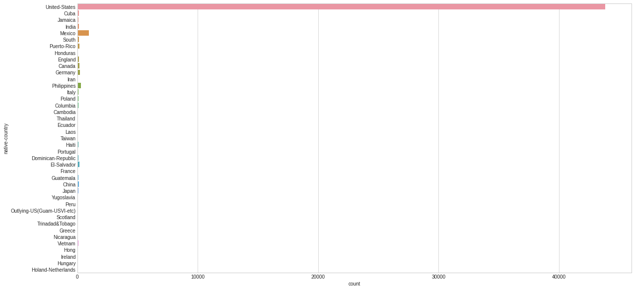
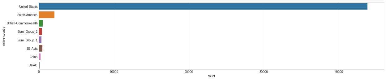
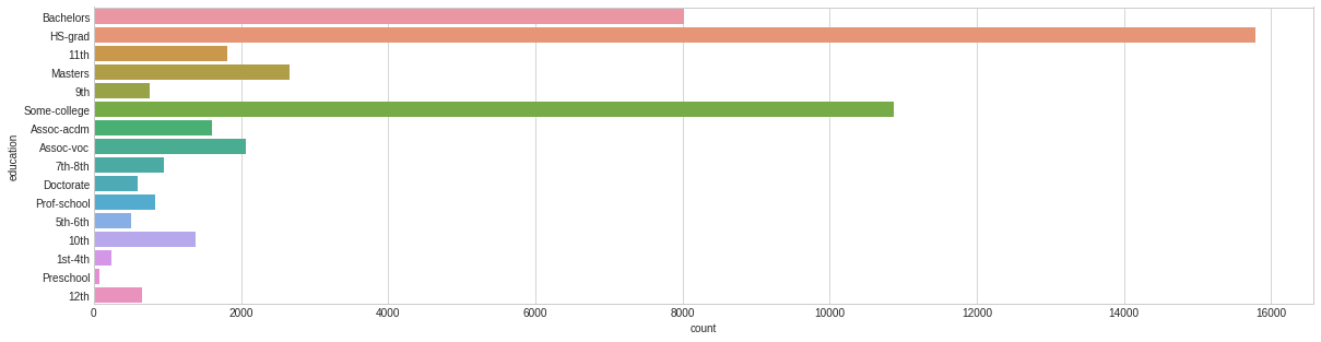
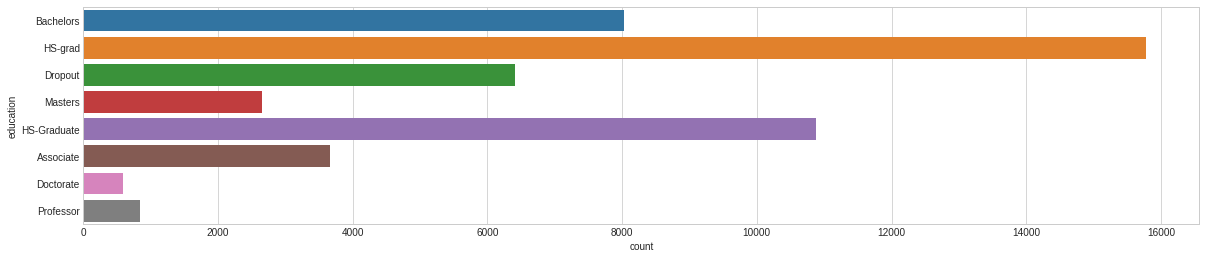
Feature Predclass
This is the feature we are trying to predict. We’ll change the string to a binary 0/1. With 1 signifying over $50K.
# Can we bucket some of these groups? plt.style.use('seaborn-whitegrid') plt.figure(figsize=(20,10)) sns.countplot(y="native-country", data=dataset_raw);
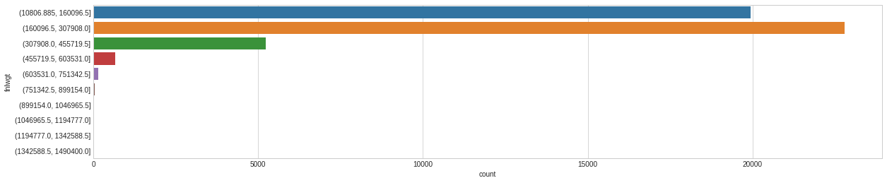
# Let's use the Pandas Cut function to bin the data in equally sized buckets dataset_bin['fnlwgt'] = pd.cut(dataset_raw['fnlwgt'], 10) dataset_con['fnlwgt'] = dataset_raw['fnlwgt']
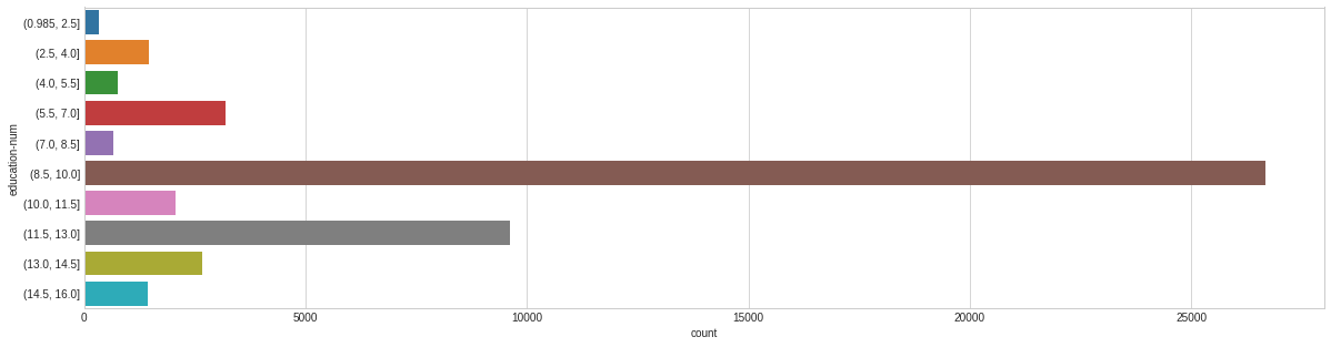
# Let's use the Pandas Cut function to bin the data in equally sized buckets dataset_bin['education-num'] = pd.cut(dataset_raw['education-num'], 10) dataset_con['education-num'] = dataset_raw['education-num']
# Let's use the Pandas Cut function to bin the data in equally sized buckets dataset_bin['hours-per-week'] = pd.cut(dataset_raw['hours-per-week'], 10) dataset_con['hours-per-week'] = dataset_raw['hours-per-week']
# Let's use the Pandas Cut function to bin the data in equally sized buckets dataset_bin['capital-gain'] = pd.cut(dataset_raw['capital-gain'], 5) dataset_con['capital-gain'] = dataset_raw['capital-gain']
# Let's use the Pandas Cut function to bin the data in equally sized buckets dataset_bin['capital-loss'] = pd.cut(dataset_raw['capital-loss'], 5) dataset_con['capital-loss'] = dataset_raw['capital-loss']
# Some features we'll consider to be in good enough shape as to pass through dataset_con['sex'] = dataset_bin['sex'] = dataset_raw['sex'] dataset_con['race'] = dataset_bin['race'] = dataset_raw['race'] dataset_con['relationship'] = dataset_bin['relationship'] = dataset_raw['relationship']
Bi-variate Analysis
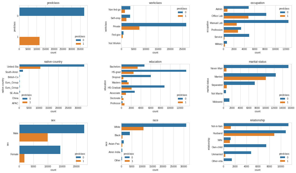
So far, we have analised all features individually. Let’s now start combining some of these features together to obtain further insight into the interactions between them.
1 2 3 4 5 6 7 8 9 10 11 12 13 14 15 16
# Plot a count of the categories from each categorical feature split by our prediction class: salary - predclass. defplot_bivariate_bar(dataset, hue, cols=5, width=20, height=15, hspace=0.2, wspace=0.5): dataset = dataset.select_dtypes(include=[np.object]) plt.style.use('seaborn-whitegrid') fig = plt.figure(figsize=(width,height)) fig.subplots_adjust(left=None, bottom=None, right=None, top=None, wspace=wspace, hspace=hspace) rows = math.ceil(float(dataset.shape[1]) / cols) for i, column in enumerate(dataset.columns): ax = fig.add_subplot(rows, cols, i + 1) ax.set_title(column) if dataset.dtypes[column] == np.object: g = sns.countplot(y=column, hue=hue, data=dataset) substrings = [s.get_text()[:10] for s in g.get_yticklabels()] g.set(yticklabels=substrings) plot_bivariate_bar(dataset_con, hue='predclass', cols=3, width=20, height=12, hspace=0.4, wspace=0.5)
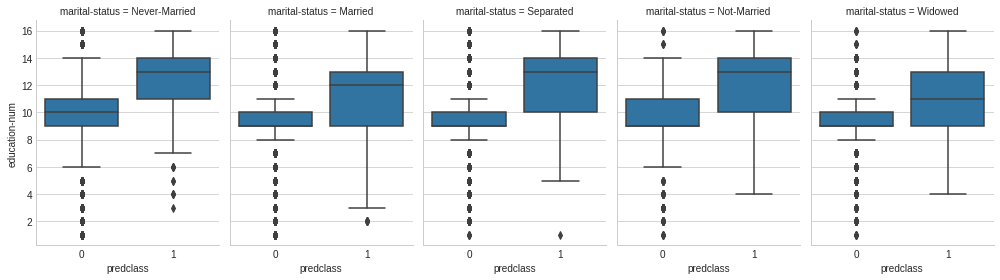
1 2 3 4
# Effect of Marital Status and Education on Income, across Marital Status. plt.style.use('seaborn-whitegrid') g = sns.FacetGrid(dataset_con, col='marital-status', size=4, aspect=.7) g = g.map(sns.boxplot, 'predclass', 'education-num')
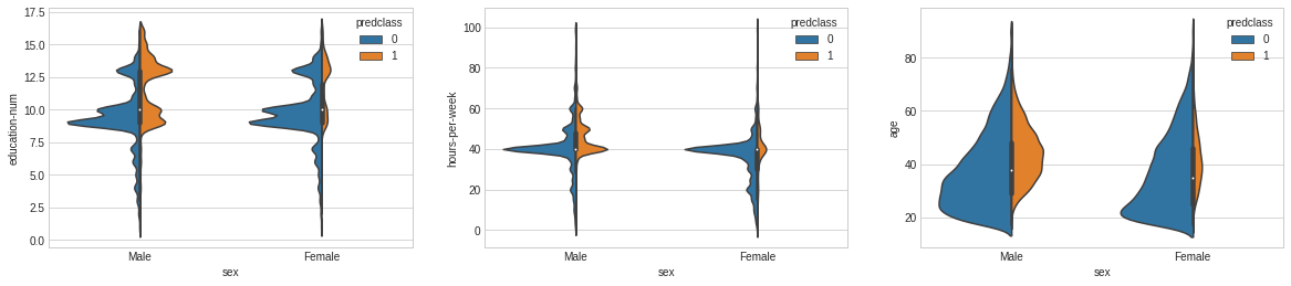
1 2 3 4 5 6 7 8 9 10 11
# Historical Trends on the Sex, Education, HPW and Age impact on Income. plt.style.use('seaborn-whitegrid') fig = plt.figure(figsize=(20,4)) plt.subplot(1, 3, 1) sns.violinplot(x='sex', y='education-num', hue='predclass', data=dataset_con, split=True, scale='count');
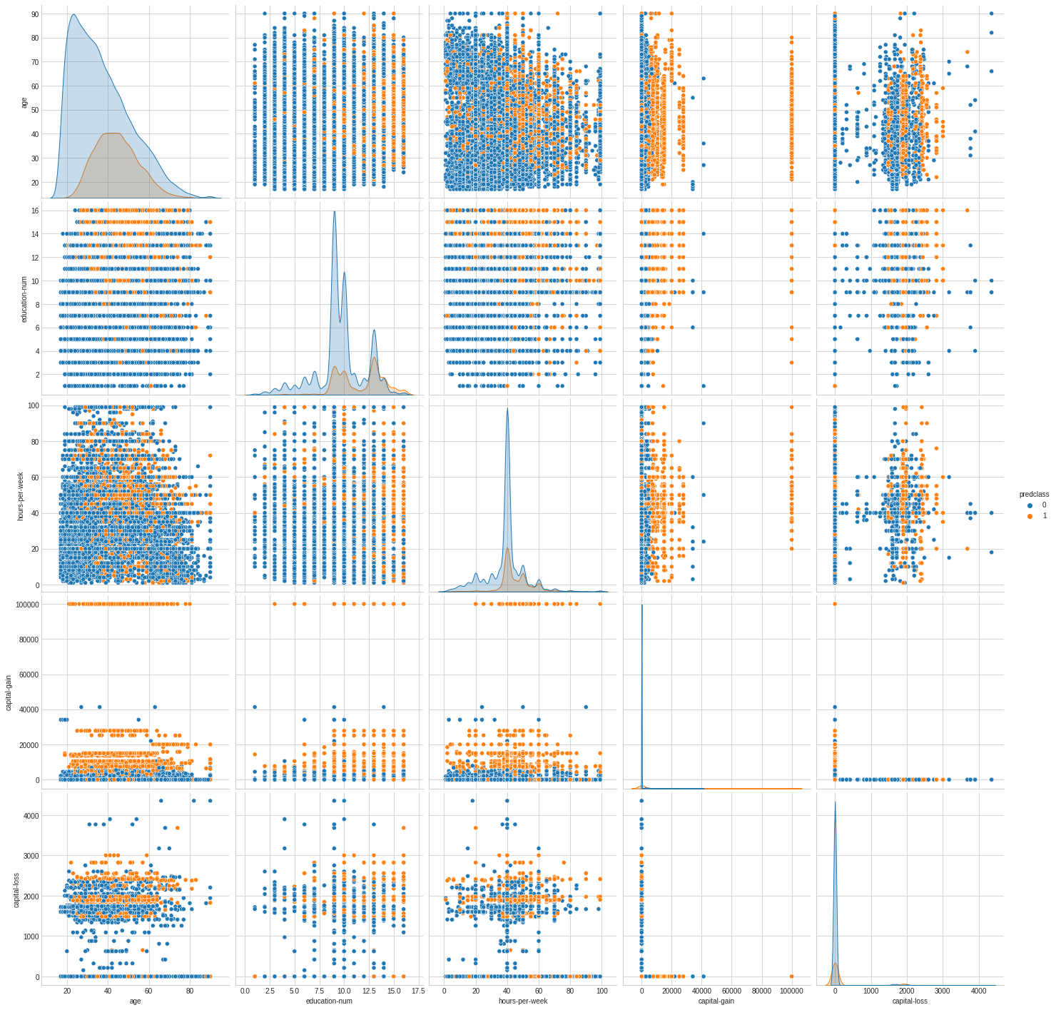
# Interaction between pairs of features. sns.pairplot(dataset_con[['age','education-num','hours-per-week','predclass','capital-gain','capital-loss']], hue="predclass", diag_kind="kde", size=4);
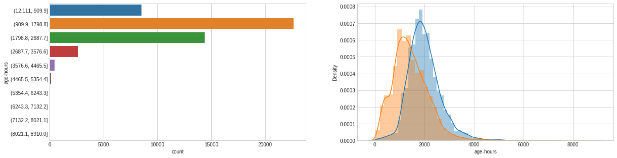
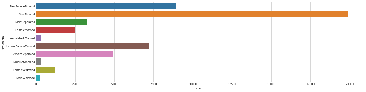
Feature Crossing: Age + Hours Per Week
So far, we have modified and cleaned features that existed in our dataset. However, we can go further and create a new new variables, adding human knowledge on the interaction between features.
1 2 3 4 5 6 7 8 9 10 11 12 13
# Crossing Numerical Features dataset_con['age-hours'] = dataset_con['age'] * dataset_con['hours-per-week']
Remember that Machine Learning algorithms perform Linear Algebra on Matrices, which means all features need have numeric values. The process of converting Categorical Features into values is called Encoding.
# One Hot Encodes all labels before Machine Learning one_hot_cols = dataset_bin.columns.tolist() one_hot_cols.remove('predclass') dataset_bin_enc = pd.get_dummies(dataset_bin, columns=one_hot_cols)
dataset_bin_enc.head()
predclass
age_(16.927, 24.3]
age_(24.3, 31.6]
age_(31.6, 38.9]
age_(38.9, 46.2]
age_(46.2, 53.5]
age_(53.5, 60.8]
age_(60.8, 68.1]
age_(68.1, 75.4]
age_(75.4, 82.7]
...
sex-marital_FemaleMarried
sex-marital_FemaleNever-Married
sex-marital_FemaleNot-Married
sex-marital_FemaleSeparated
sex-marital_FemaleWidowed
sex-marital_MaleMarried
sex-marital_MaleNever-Married
sex-marital_MaleNot-Married
sex-marital_MaleSeparated
sex-marital_MaleWidowed
0
0
0
0
0
1
0
0
0
0
0
...
0
0
0
0
0
0
1
0
0
0
1
0
0
0
0
0
1
0
0
0
0
...
0
0
0
0
0
1
0
0
0
0
2
0
0
0
1
0
0
0
0
0
0
...
0
0
0
0
0
0
0
0
1
0
3
0
0
0
0
0
1
0
0
0
0
...
0
0
0
0
0
1
0
0
0
0
4
0
0
1
0
0
0
0
0
0
0
...
1
0
0
0
0
0
0
0
0
0
5 rows × 116 columns
1 2 3 4 5 6 7 8 9 10 11 12 13 14 15 16 17
# 'dataset_con' is original input dataset for this section
# build a new dataframe containing only the object columns
# delete the rows contains NaN values dataset_con_enc = dataset_con.dropna(axis=0) print(dataset_con_enc) dataset_con_enc[dataset_con_enc.isnull().any(axis=1)]
predclass age workclass occupation native-country education \
0 0 39 Non-fed-gov Admin United-States Bachelors
1 0 50 Self-emp Office Labour United-States Bachelors
2 0 38 Private Manual Labour United-States HS-grad
3 0 53 Private Manual Labour United-States Dropout
4 0 28 Private Professional South-America Bachelors
... ... ... ... ... ... ...
48836 0 33 Private Professional United-States Bachelors
48837 0 39 Private Professional United-States Bachelors
48839 0 38 Private Professional United-States Bachelors
48840 0 44 Private Admin United-States Bachelors
48841 1 35 Self-emp Office Labour United-States Bachelors
marital-status fnlwgt education-num hours-per-week capital-gain \
0 Never-Married 77516 13 40 2174
1 Married 83311 13 13 0
2 Separated 215646 9 40 0
3 Married 234721 7 40 0
4 Married 338409 13 40 0
... ... ... ... ... ...
48836 Never-Married 245211 13 40 0
48837 Separated 215419 13 36 0
48839 Married 374983 13 50 0
48840 Separated 83891 13 40 5455
48841 Married 182148 13 60 0
capital-loss sex race relationship age-hours \
0 0 Male White Not-in-family 1560
1 0 Male White Husband 650
2 0 Male White Not-in-family 1520
3 0 Male Black Husband 2120
4 0 Female Black Wife 1120
... ... ... ... ... ...
48836 0 Male White Own-child 1320
48837 0 Female White Not-in-family 1404
48839 0 Male White Husband 1900
48840 0 Male Asian-Pac-Islander Own-child 1760
48841 0 Male White Husband 2100
sex-marital
0 MaleNever-Married
1 MaleMarried
2 MaleSeparated
3 MaleMarried
4 FemaleMarried
... ...
48836 MaleNever-Married
48837 FemaleSeparated
48839 MaleMarried
48840 MaleSeparated
48841 MaleMarried
[45222 rows x 17 columns]
predclass
age
workclass
occupation
native-country
education
marital-status
fnlwgt
education-num
hours-per-week
capital-gain
capital-loss
sex
race
relationship
age-hours
sex-marital
1 2 3 4 5
# Label Encode all labels le = preprocessing.LabelEncoder() dataset_con_enc = dataset_con_enc.apply(le.fit_transform)
dataset_con_enc.head()
predclass
age
workclass
occupation
native-country
education
marital-status
fnlwgt
education-num
hours-per-week
capital-gain
capital-loss
sex
race
relationship
age-hours
sex-marital
0
0
22
1
0
7
1
1
3217
12
39
26
0
1
4
1
655
6
1
0
33
4
3
7
1
0
3519
12
12
0
0
1
4
0
302
5
2
0
21
3
1
7
5
3
17196
8
39
0
0
1
4
1
644
8
3
0
36
3
1
7
3
0
18738
6
39
0
0
1
2
0
847
5
4
0
11
3
4
6
1
0
23828
12
39
0
0
0
2
5
494
0
Feature Reduction / Selection
Once we have our features ready to use, we might find that the number of features available is too large to be run in a reasonable timeframe by our machine learning algorithms. There’s a number of options available to us for feature reduction and feature selection.
Dimensionality Reduction:
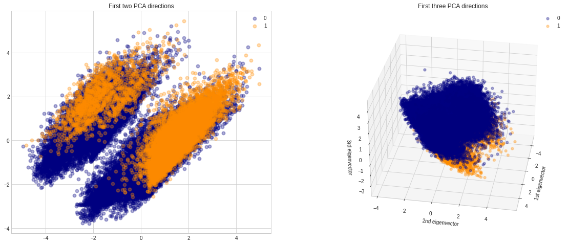
Principal Component Analysis (PCA): Principal component analysis (PCA) is a statistical procedure that uses an orthogonal transformation to convert a set of observations of possibly correlated variables into a set of values of linearly uncorrelated variables called principal components. This transformation is defined in such a way that the first principal component has the largest possible variance (that is, accounts for as much of the variability in the data as possible), and each succeeding component in turn has the highest variance possible under the constraint that it is orthogonal to the preceding components.
Singular Value Decomposition (SVD): SVD is a factorization of a real or complex matrix. It is the generalization of the eigendecomposition of a positive semidefinite normal matrix (for example, a symmetric matrix with positive eigenvalues) to any m×n matrix via an extension of the polar decomposition. It has many useful applications in signal processing and statistics.
Feature Importance/Relevance:
Filter Methods: Filter type methods select features based only on general metrics like the correlation with the variable to predict. Filter methods suppress the least interesting variables. The other variables will be part of a classification or a regression model used to classify or to predict data. These methods are particularly effective in computation time and robust to overfitting.
Wrapper Methods: Wrapper methods evaluate subsets of variables which allows, unlike filter approaches, to detect the possible interactions between variables. The two main disadvantages of these methods are : The increasing overfitting risk when the number of observations is insufficient. AND. The significant computation time when the number of variables is large.
Embedded Methods: Embedded methods try to combine the advantages of both previous methods. A learning algorithm takes advantage of its own variable selection process and performs feature selection and classification simultaneously.
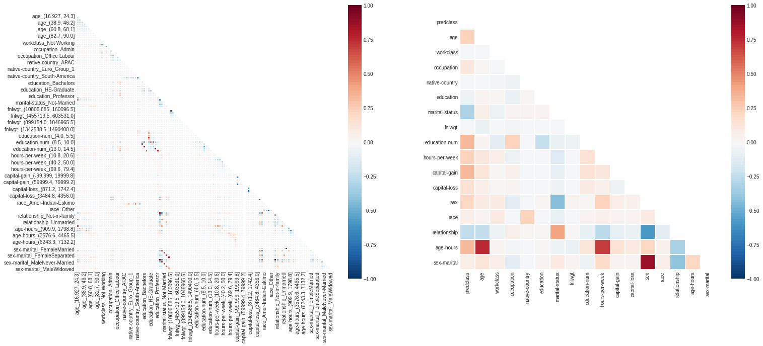
Feature Correlation
Correlation ia s measure of how much two random variables change together. Features should be uncorrelated with each other and highly correlated to the feature we’re trying to predict.
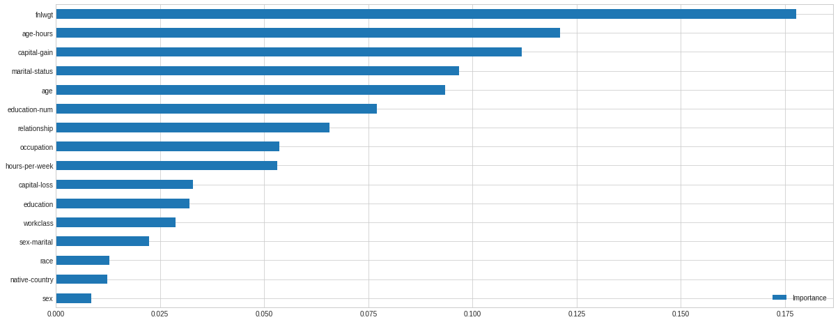
Random forest consists of a number of decision trees. Every node in the decision trees is a condition on a single feature, designed to split the dataset into two so that similar response values end up in the same set. The measure based on which the (locally) optimal condition is chosen is called impurity. When training a tree, it can be computed how much each feature decreases the weighted impurity in a tree. For a forest, the impurity decrease from each feature can be averaged and the features are ranked according to this measure. This is the feature importance measure exposed in sklearn’s Random Forest implementations.
1 2 3 4 5 6 7 8
# Using Random Forest to gain an insight on Feature Importance clf = RandomForestClassifier() clf.fit(dataset_con_enc.drop('predclass', axis=1), dataset_con_enc['predclass'])
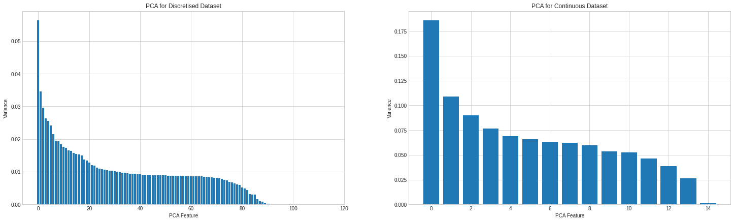
Principal component analysis (PCA) is a statistical procedure that uses an orthogonal transformation to convert a set of observations of possibly correlated variables into a set of values of linearly uncorrelated variables called principal components. This transformation is defined in such a way that the first principal component has the largest possible variance (that is, accounts for as much of the variability in the data as possible), and each succeeding component in turn has the highest variance possible under the constraint that it is orthogonal to the preceding components.
We can use PCA to reduce the number of features to use in our ML algorithms, and graphing the variance gives us an idea of how many features we really need to represent our dataset fully.
# Calculating PCA for both datasets, and graphing the Variance for each feature, per dataset std_scale = preprocessing.StandardScaler().fit(dataset_bin_enc.drop('predclass', axis=1)) X = std_scale.transform(dataset_bin_enc.drop('predclass', axis=1)) pca1 = PCA(n_components=len(dataset_bin_enc.columns)-1) fit1 = pca1.fit(X)
# PCA's components graphed in 2D and 3D # Apply Scaling std_scale = preprocessing.StandardScaler().fit(dataset_con_enc.drop('predclass', axis=1)) X = std_scale.transform(dataset_con_enc.drop('predclass', axis=1)) y = dataset_con_enc['predclass']
pca = PCA(n_components=3) X_reduced = pca.fit(X).transform(X) for color, i, target_name in zip(colors, [0, 1], target_names): ax.scatter(X_reduced[y == i, 0], X_reduced[y == i, 1], X_reduced[y == i, 2], color=color, alpha=alpha, lw=lw, label=target_name) plt.legend(loc='best', shadow=False, scatterpoints=1) ax.set_title("First three PCA directions") ax.set_xlabel("1st eigenvector") ax.set_ylabel("2nd eigenvector") ax.set_zlabel("3rd eigenvector")
# rotate the axes ax.view_init(30, 10)
Recursive Feature Elimination
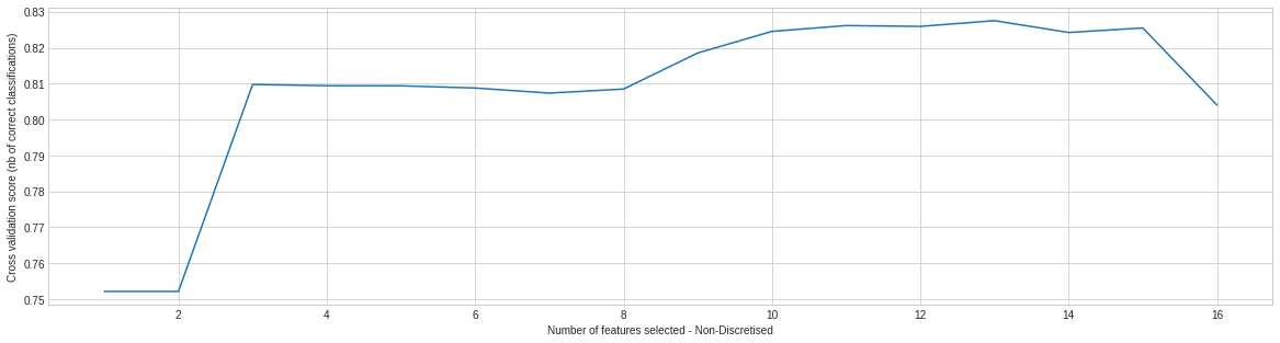
Feature ranking with recursive feature elimination and cross-validated selection of the best number of features.
1 2 3 4 5 6 7 8 9 10 11 12 13 14
# Calculating RFE for non-discretised dataset, and graphing the Importance for each feature, per dataset selector1 = RFECV(LogisticRegression(), step=1, cv=5, n_jobs=-1) selector1 = selector1.fit(dataset_con_enc.drop('predclass', axis=1).values, dataset_con_enc['predclass'].values) print("Feature Ranking For Non-Discretised: %s" % selector1.ranking_) print("Optimal number of features : %d" % selector1.n_features_) # Plot number of features VS. cross-validation scores plt.style.use('seaborn-whitegrid') plt.figure(figsize=(20,5)) plt.xlabel("Number of features selected - Non-Discretised") plt.ylabel("Cross validation score (nb of correct classifications)") plt.plot(range(1, len(selector1.grid_scores_) + 1), selector1.grid_scores_);
# Feature space could be subsetted like so: dataset_con_enc = dataset_con_enc[dataset_con_enc.columns[np.insert(selector1.support_, 0, True)]]
Feature Ranking For Non-Discretised: [1 1 1 1 3 1 4 1 1 1 1 1 1 1 2 1]
Optimal number of features : 13
Selecting Dataset
We now have two datasets to choose from to apply our ML algorithms. The one-hot-encoded, and the label-encoded. For now, we have decided not to use feature reduction or selection algorithms.
# Change the dataset to test how would the algorithms perform under a differently encoded dataset.
selected_dataset = dataset_bin_enc
1
selected_dataset.head(2)
predclass
age_(16.927, 24.3]
age_(24.3, 31.6]
age_(31.6, 38.9]
age_(38.9, 46.2]
age_(46.2, 53.5]
age_(53.5, 60.8]
age_(60.8, 68.1]
age_(68.1, 75.4]
age_(75.4, 82.7]
...
sex-marital_FemaleMarried
sex-marital_FemaleNever-Married
sex-marital_FemaleNot-Married
sex-marital_FemaleSeparated
sex-marital_FemaleWidowed
sex-marital_MaleMarried
sex-marital_MaleNever-Married
sex-marital_MaleNot-Married
sex-marital_MaleSeparated
sex-marital_MaleWidowed
0
0
0
0
0
1
0
0
0
0
0
...
0
0
0
0
0
0
1
0
0
0
1
0
0
0
0
0
1
0
0
0
0
...
0
0
0
0
0
1
0
0
0
0
2 rows × 116 columns
Splitting Data into Training and Testing Datasets
We need to split the data back into the training and testing datasets. Remember we joined both right at the beginning.
1
2
3
# Splitting the Training and Test data sets train = selected_dataset.loc[0:32560,:] test = selected_dataset.loc[32560:,:]
Removing Samples with Missing data
We could have removed rows with missing data during feature cleaning, but we’re choosing to do it at this point. It’s easier to do it this way, right after we split the data into Training and Testing. Otherwise we would have had to keep track of the number of deleted rows in our data and take that into account when deciding on a splitting boundary for our joined data.
1 2 3 4
# Given missing fields are a small percentange of the overall dataset,
# we have chosen to delete them.
train = train.dropna(axis=0)
test = test.dropna(axis=0)